Boundary condition specification for multiphase simulations in Simcenter STAR-CCM+

Have you ever intended to run a multiphase simulation in Simcenter STAR-CCM+ and found that once you thought everything was set up properly, once all initial conditions and boundary conditions where specified, the simulation never started because some sum of mass or mole fractions did not add up to unity? I have experienced this, and even though I work daily with Simcenter STAR-CCM+, this still happens to me. My idea with this blog post is to sort out the different settings for the different types of multiphase simulations.

Eulerian models

The difficulty generally stems from the different settings in reference to the Eulerian models. In Simcenter STAR-CCM+ we have the following Eulerian multiphase models:

EMP – Eulerian multiphase model, the mother of Eulerian simulations. The most versatile model, but also the most expensive Eulerian model.
MMP – Mixture Multiphase model, a simplification of the EMP model that assumes some homogeneity.
DMP – A real lightweight Eulerian model that simulates highly diluted dispersed phases with small impact to the continuous flow. (Preferably less than 1% volume fraction)
VOF – Volume of fluid, an interface tracking model for simulation of immiscible fluids.

You can read more about multiphase modelling capabilities in our previous blog post via this link. These models are somewhat treated differently when it comes to settings. In terms of how advanced the settings are, I will classify the models like members of a family. VOF and MMP models are siblings (the teenagers), while the EMP model (the mother) is seen as separate and the DMP has special treatment (the unruly small child).

There are different reasons for having specific settings at different locations, some are not necessarily intuitive, and some might come to shift in the future. In the last years, hybrid multiphase modelling has been given large focus, and a lot of effort is put into hybrid multiphase implementations. This has led to more and more inputs in a simulation, where the differences between the models become more apparent. And the risk of losing track of the differences can lead to some frustration. Hopefully some of this confusion can be sorted out with this blog post. Below we will investigate an example, set up with the different models, to highlight where to specify the settings.

The example

The best way to show the differences in the setups is to create simulations for each model with as similar setups as possible. So, for comparison, this is the settings that are the same for the different models:

A two-phase system
A multi-component liquid phase with water (H2O) and methanol (CH4O)
A multi-component gas with oxygen (O2) and carbon dioxide (CO2)
Initial and boundary conditions (inlet/outlet) is species mass fraction 0.99 for water and 0.01 for methanol, for the liquid phase.
Initial and boundary conditions (inlet/outlets) are species mass fraction 0.95 for oxygen and 0.05 for carbon dioxide, for the gas phase.
Initial and boundary conditions for the volume fractions is 0.5 for the liquid phase and 0.5 for the gas phase.
Note that the values and setup is nonsensical, especially since VOF fractions should be separated by an interface, either by specifying full fractions to different locations or by starting with one phase and filling up with another. (Imagine a pouring liquid.)
Note also that the DMP model has special treatment since it does not allow for a multi-component phase. It has been specified as pure water in a multi-component gas as the continuous phase.
No specific regard has been put into including multiphase interaction models, more than to show where special attention is needed in a similar setup.

The example with VOF

Instead of describing the differences in text, a picture of the simulation tree is shown and settings in reference to the model type is highlighted. The volume fractions initial conditions for the VOF-model are located under the continua. The species mass fraction for each component is specified under each separate Eulerian phase.

The left side shows the model selection for the VOF-model for reference. The inlet conditions for the species mass fractions are specified under phase conditions while the volume fractions are specified as physics values for the inlet boundary. Note also that momentum and source options are specified as phase conditions while volume fractions are specified under physics conditions.

The example with EMP

The EMP model setup is unique as an Eulerian model in Simcenter STAR-CCM+ as it is the only one where both the initial conditions and inlet/outlet conditions for both species mass fraction and phase volume fraction is specified as phase specific. This is evident from the two pictures below.

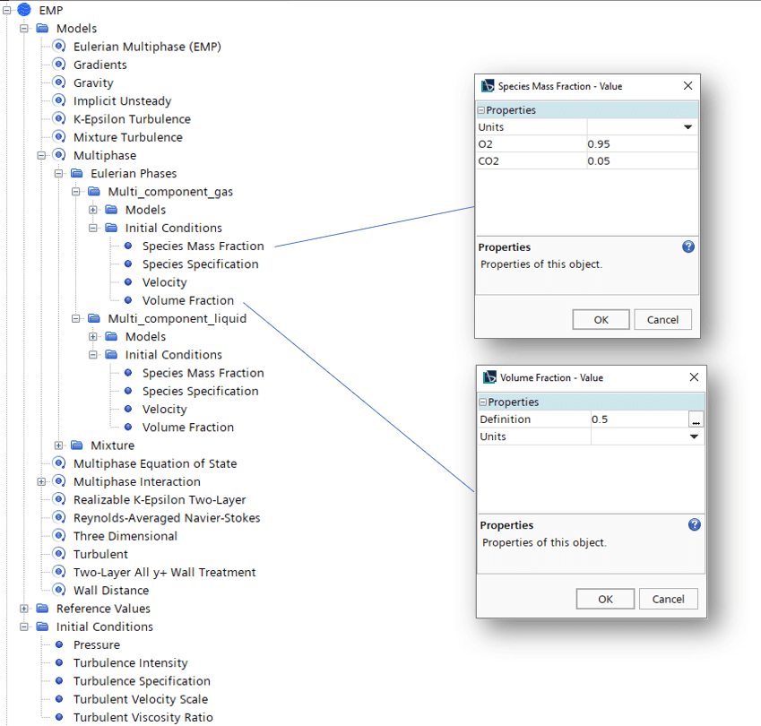
Note also that all options for sources are specified as phase conditions.

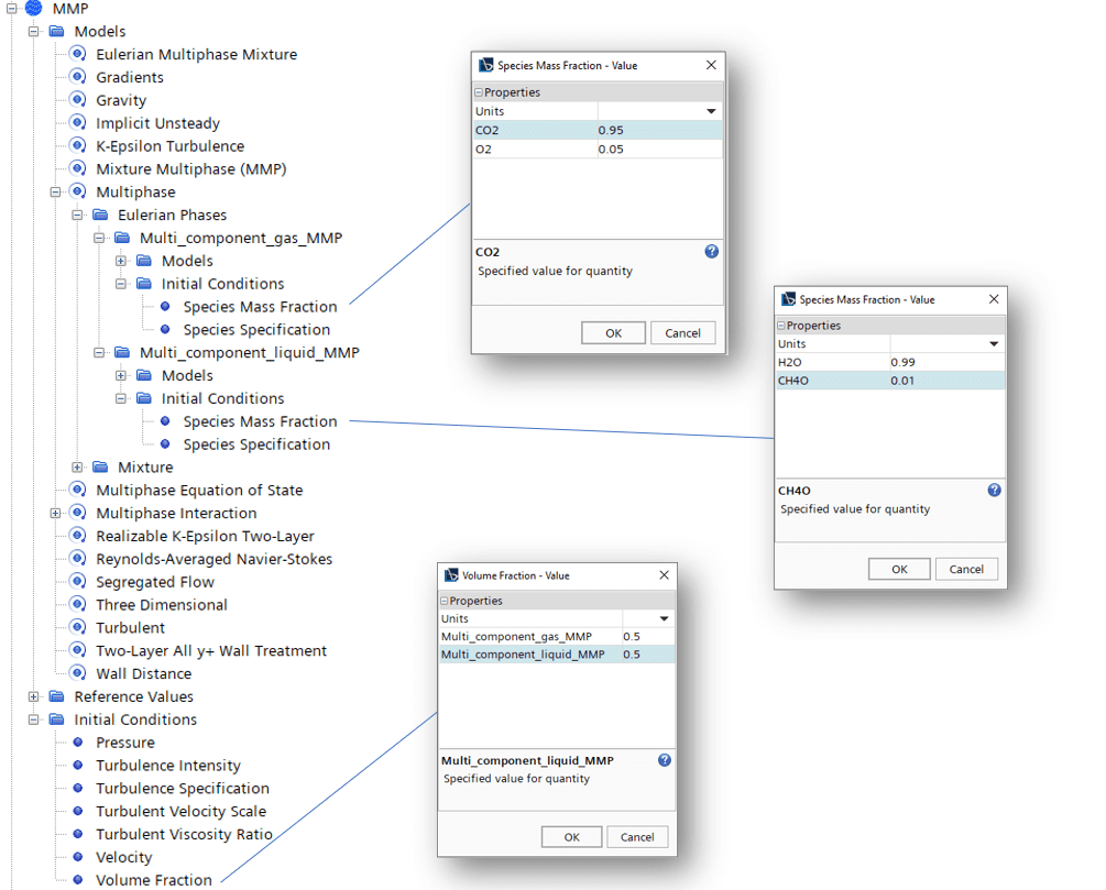
The example with MMP

As mentioned above the MMP model has very similar options to the VOF setup. Initial conditions for the species mass fractions and phase volume fractions are separated in the same manner. The inlet boundary conditions for species, volume fractions and momentum source options are also separated in the same way, as can be seen in the pictures below.

When it comes to the MMP model there is another setting worth mentioning. When it comes to a mixture simulation, it is likely that you want the phases to be able to move at different velocities, and that you want to include slip velocity. The slip velocity can be activated as a phase interaction between phases. However, the selection of the slip model does not automatically include it since the default value for the interaction-model is “no-slip”. It requires a separate selection, and that selection appears as a selection of phase interaction under the phase conditions for the region. The picture below shows where the selections are made.

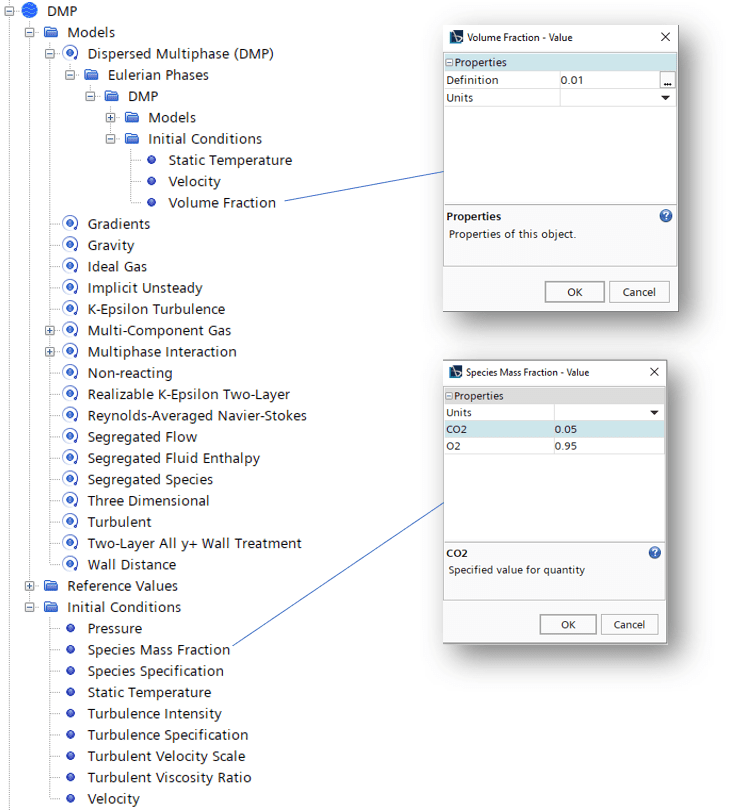
The example with DMP

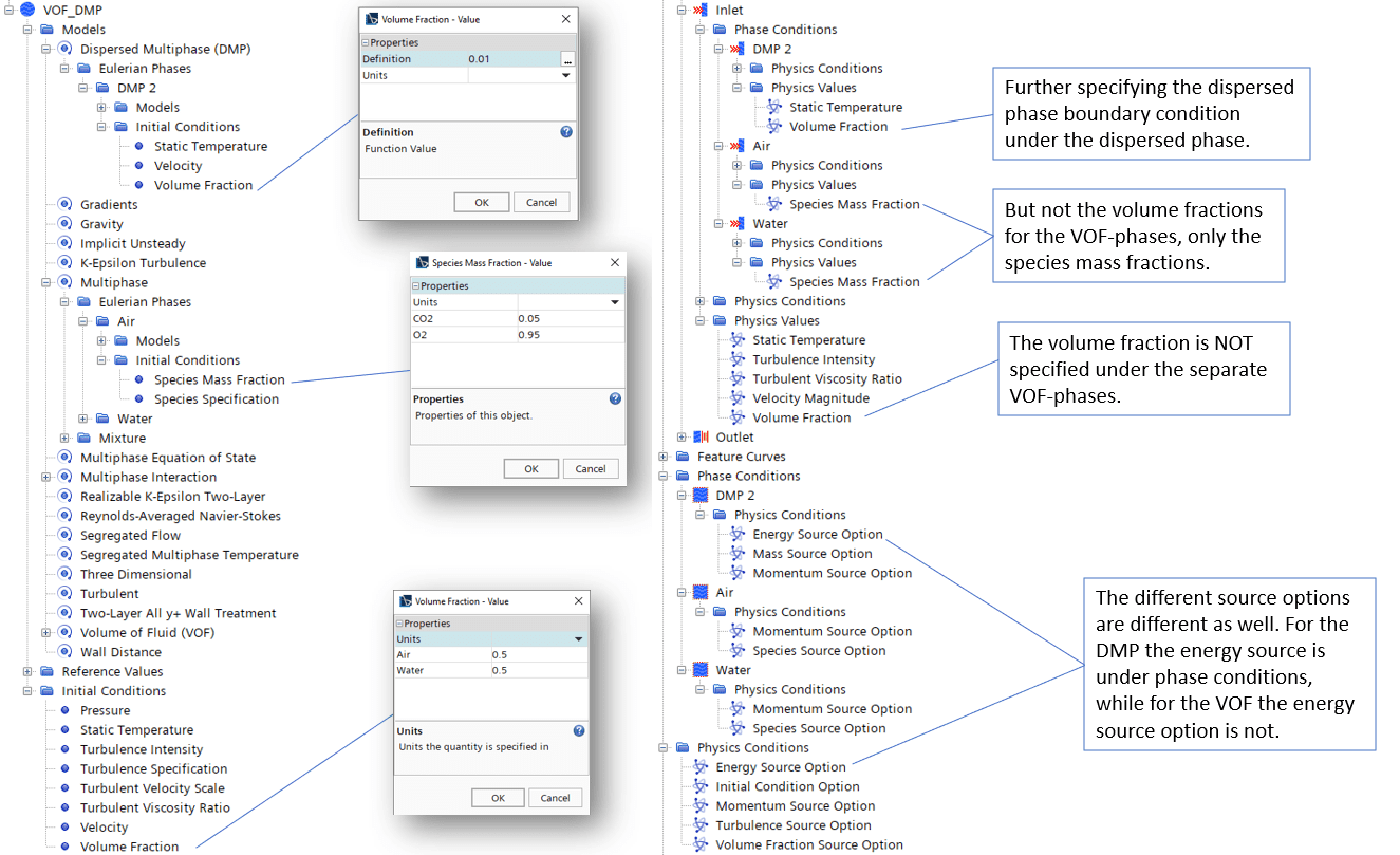
As mentioned above the DMP model is a lightweight model when it comes to Eulerian multiphase modelling. The method does not permit the dispersed phase to be multicomponent. So, in the example the liquid phase is the dispersed phase, set to pure water.

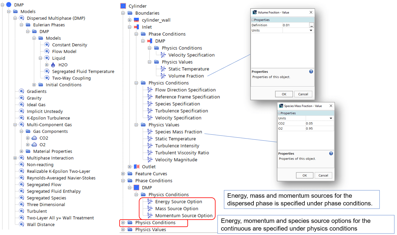
The species mass fractions for the gas phase here is moved down to continuum initial conditions and is not located under any type of phase. Instead, you specify the fractions for the continuous phase as if the simulations only contained one phase. The addition of the dispersed phase is then specified under the DMP node in the model tree. When looking at the inlet conditions for the DMP simulation, you only specify the volume fraction of the dispersed phase. There is no requirement for unity over a summation of volume fractions. Because the DMP volume fraction implies that the continuous phase covers the rest. The sources specification for the dispersed phase is located under phase conditions.

Hybrid multiphase modelling

The above examples show the models in the forms they have, when simulated separately. In hybrid multiphase modelling we combine a set of multiphase models to expand the range of physics we want to cover. Granted that hybrid multiphase modelling has been implemented in the last couple of years, the settings for this type of combinatory models are not necessarily uniform, and may be addressed later. Imagine a simulation where you wish to include two phases and for that we use VOF, a liquid phase and gas phase. We use the same example as above in our VOF example. With the addition of a DMP phase, here representing dispersed water (in a real simulation the dispersed water would be in the gas-phase, but for the sake of the setup here, there is no need to separate the DMP phase from the liquid VOF phase). Setting this up looking at the initial conditions and the inlet conditions in the picture below we can see why it is easy to get confused.

The lower initial conditions for the VOF-phase need to abide to the summation to unity, while the dispersed phase volume fraction, specified under the initial conditions for the Eulerian phases (those for the DMP model) does not have to follow the summation convention. It is the same with the inlet conditions, fractions for the VOF-phases are specified under the inlet directly while the DMP phase is specified as a phase condition.

There are more examples of where the convention might be a bit confusing. One example is when you have a 3-phase system of air, water and steam and wish to include Spalding evaporation/condensation in a MMP simulation. The Spalding evaporation model does not support single component, meaning that you need to have a multicomponent phase of the phases taking part in that phase change. But you can have a multi-component phase with only one specified component. This is somewhat non-intuitive by itself. But it gets really confusing when the default fraction of a multicomponent phase is zero, regardless of the number of components. Meaning that the default initial conditions for all the phases and boundary conditions associated with the inlets are zero. Not only is the volume fraction zero, but once specified the mass fraction in that phase is also zero.

I hope this will help you sort out the differences and in the least give you a hint to where to start looking when you initialize your simulation and get the report that somewhere sum of mass fractions does not add up to unity. As usual, reach out to support@volupe.com with any questions.