Electromagnetism in Simcenter STAR-CCM+ with symmetric boundaries for magnetic simulations

Simcenter STAR-CCM+ is a multiphysics tool capable of simulating a wide range of different physical aspects. One of these areas of simulation is electromagnetism (EMAG), which we are going to look closer at in this week’s blog post at the Volupe blog.

What is electromagnetism?

Electromagnetics involves modelling of electrostatics (solves for electric potential due to how dense the electric charge in the system is), electric currents (solved with electrodynamic potential models) and magnetism (magnetic fields, induces by permanent magnets or coils – for example).

The physical phenomenon of electromagnetism is described by Maxwell’s equations, which are a set of coupled partial differential equations for the electric (E) and the magnetic (B) fields. The equations are shown in the picture below [1].

Modelling electromagnetics

As for the Navier-Stokes equations, which also are a set of coupled partial differential equations, the solution to Maxwell’s equations must be iterated. There are a lot of similarities between solving for electromagnetics and fluid flow. Solving for current can be compared to solving for velocity, and solving for potential in the electromagnetic field can be compared to solving for pressure in fluid flow. Knowing this analogy, it might be easier to grasp what is happening in your EMAG simulation – and how to evaluate the results of your simulations.

When running electromagnetic simulations, it is recommended to use the double precision version of the software (version R8) to maintain numerical accuracy. Some other tips can be to avoid resolving the mesh too much in the areas (usually corners) where you have a discontinuance (change) in boundary conditions (to avoid obtaining singularities in the solution), and also to use tetrahedral mesher since the solver is based on finite elements (calculations are done by FEM).

How to model magnetic simulations with symmetric boundaries

If you narrow the simulation down to only looking at the magnetic part of the simulation you might be interested in looking at just a part of a longer magnet, then symmetry planes are handy to use. In flow simulations it is enough to specify “symmetry” as boundary condition, but in magnetic simulations you also have to specify in what way you have symmetry. To allow the magnetic field to behave symmetric (or repeating), you should select either “Insulating” or “Anti-symmetry – Perfect electric conductor”, since these boundary conditions do not allow for current eddies to cross the boundary. The magnetic flux is not allowed to cross any boundary either, so it is only the magnetic potential (which is always orthogonal against the flux) that is allowed to cross the boundaries. In the image below, taken from Simcenter STAR-CCM+’s documentation, the boundary conditions are explained in more detail.

From the picture above you can categorize the symmetry boundary condition to be of type Neumann, the anti-symmetry (and insulating) to be of type Dirichlet, and you also have the gap boundary condition to model thin virtual air gaps. Notice that you can also specify the magnetization direction at the boundaries, which describes the magnetic flux direction for each boundary. The magnetic direction will indicate in which direction you have the north side of the magnet.

Example – modelling magnetic fields with symmetry planes for infinite rods

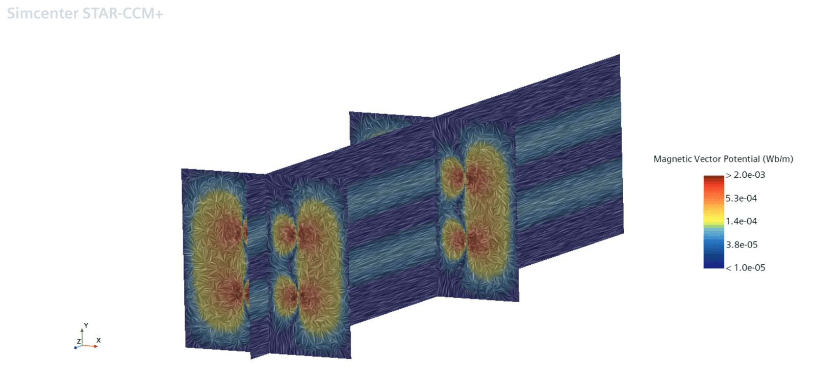
In the example discussed in this section, we will look at the simulation of four magnetic rods, highlighted in pink/purple in the picture below.

The rods are modelled as permanent magnets and in the picture below the magnetic flux density is visualized. The magnetization direction for all rods is in positive y-direction.

By visualizing the magnetic vector potential, you can see that the solution is identical regardless of which 2D-cross-section (XY) plane you are looking at in z-direction. Which is due to the boundary condition “Anti-symmetric – perfect electric conductor” at all the outer boundaries of the computational domain – in order to model symmetry at the outer boundaries.

If you instead would have used the symmetric boundary condition for perfect magnetic conduction you would have obtained a non-symmetric magnetic field downstream along the rods. This magnetic field would not have propagated straight out of the domain either, which can be misleading since the name of the boundary condition is implying symmetry.

This week’s post is published today (Wednesday) since tomorrow (Thursday) is a public holiday in Sweden, and Friday is therefore a ”squeeze day” in many countries. Most people do therefore have a holdiday from work, but we at Volupe will of course not close completely, so you are welcome to reach out to us as usual at support@volupe.com.

We hope that this blog post has been of interest, and that it will help you in your future electromagnetic simulations. Wishing you a nice and long weekend!