This week’s blog post will be about heat transfer, in general the environment boundary condition in Simcenter STAR-CCM+ and its benefits. There will also be a small deep dive into multi-layer resistance and the limitations of thermal resistance on an outer boundary for this feature.

We have previously gone over some tips and tricks and some considerations when it comes to the capability of simulating radiation. Some consideration is given to radiation also regarding the Environment boundary condition, but focus is going to be on how to consider insulation, radiation will not be explicitly exemplified.

The environment boundary condition

The environment boundary condition was used in the examples regarding surface-to-surface radiation (S2S) and the details regarding this can be read here [S2S radiation in Simcenter STAR-CCM+ – VOLUPE Software]. As in the example where the environment boundary condition can be used to include external radiation properties and once activated will allow you select radiative properties, both internally and externally. Note also that this environment boundary condition can be used with the solar load model.

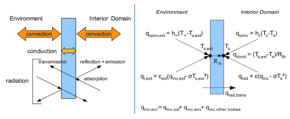
The idea of the environment boundary condition is to model the external effects to a geometry without the need for actual spatial discretisation of the immediate surroundings. Instead, all effects are modelled directly on the boundary. You typically set the Heat Transfer Coefficient together with an ambient temperature to calculate convective heat flux, weather it is forced or natural convection. That is decided in the size of the HTC.

The picture below describes the physics and the modelling for the environment boundary condition. So far, the convection and radiation are mentioned. Further, also the conduction through a boundary can be of interest. The boundary can have any finite thermal resistance, including zero. Later, that is what we will focus on when looking at multi-layer resistance.

Thermal resistance

As one option for the environment boundary condition you can specify the thermal resistance, this is exclusively for the thermal boundary condition. The physical effect of the thermal resistance shall correspond to insulation of your external boundary. The specific options for method, shown in the picture below, are the common selections of constant, field function and a number of different tables. In addition, the Multi-layer Resistance option can be used. More on that later, first we need to consider what the thermal resistance means, and what theoretical formulations there are for thermal resistance.

Formulations for thermal resistance

When it comes to describing thermal resistance, you might see three different units. The first one is [K/W] (Kelvin per Watt) and that is referred to as Absolute thermal resistance, and describes the property of a component, like a heat sink. The second one is [K∙m/W] (Kelvin and meter per Watt) and is referred to as Specific thermal resistance or thermal resistivity and is a material constant. It is in fact the reciprocal of thermal conductivity. The third one is [K∙m²/W] (Kelvin and meter squared per W) is referred to as thermal insulance and is the thermal resistance of unit area of a material. The “of unit area” is important here and gives some geometric limitations to the multi-layer resistance model.

Multi-Layer resistance

So, as described, the environment boundary condition allows for the selection of Multi-layer resistance model for thermal resistance. It is important to understand the difference in specification for the options of constant value compared to Multi-Layer resistance. In the Multi-Layer Resistance model, the user inputs are according to the picture below: Number of Layers (hence “multi-layer”), the Thickness of Each Layer and the Conductivity of Each Layer (the inverse of the specific thermal resistance). All these properties together then gives a resulting thermal insulance. Note that we have not considered the geometry or shape of the boundary to which the environment boundary condition is applied.

For a constant value you specify the thermal insulation directly, implying that you have already considered the unit area of the material. The formulation for the Multi-Layer resistance representation holds if you are interested in a flat wall. And of course, the relative error to the calculation decreases as the inner and outer diameter of the insulation layers are relatively close to each other (thin layer of insulation compared to pipe radius).

Pipe insulation calculations

To calculate the thermal resistance of each layer of insulation in a cylindrical pipe you need to use the following formulation:

Also note that, the thermal conductivity (λ) is temperature dependent and should be selected for the average temperature for that specific layer of insulation. The thermal conductivity can be both increasing and decreasing with temperature depending on material. But as the dependence is usually relatively small, for the sake of this article we treat them as constant.

The relationship between conductivity and thermal resistance of several layers of insulation (in series) is calculated according to the below formula:

The total thermal resistance in a serial problem is the sum of the individual resistances. And the resulting thermal conductivity can be obtained from the formula above.

Using Multi-Layer or simulating the insulation

The last formulation (the serial approach) is also what gives the net resistance for the Multi-Layer resistance model in Simcenter STAR-CCM+. Meaning that instead of including the effect of an increasing area as is the case in a pipe as you travel outward from the center, the area is treated as constant and only thickness is considered. Leaving the simulation with an inherent error. As described before, it is relatively small if the insulation is thin. There are a couple of approaches here in terms of doing this in your simulation. First you can ignore the error and still use the approach, baring in mind that whatever gives you a conservative result is still relevant. The other option is to calculate the net resistance for your pipe insulation layers with the logarithmic expression. And then sum up the total thermal resistance with the knowledge that the total value is the sum of each layer’s individual value. The third option is to include the insulation in your simulation. There can of course be many reasons why insulation effects are estimated instead of modelled, e.g. cell count and complexity of the simulation.

In the example below is a simple test that will show the difference in result when using either the Multi-Layer resistance model or including the actual insulation. The picture describes the case and the results. Worth adding is that the case was a simple metal ring with a set temperature as inside boundary condition. The insulation layers are 1 cm thick and the thermal conductivity of the insulation is 0.038 [W/m∙K]. From the graph it is shown that the Multi-Layer resistance approach gets less accurate when insulation thickness increases. This is due to that the Multi-Layer resistance does not take into account the increased area of the insulation when diameter is increased. Note that the relative error is what it is growing, even if the absolute difference seem to be constant. The higher the temperature gradient, the higher the absolute error becomes.

I hope this has been useful and can help you to decide what approach to use when it comes to simulating insulation and thermal resistances in Simcenter STAR-CCM+. As usual do not hesitate to reach out with any questions to support@volupe.com.