How to setup Rigid Body Motion (RBM) and Moving Reference Frame (MRF) simulations in Simcenter STAR-CCM+

In this week’s blog post we will show two different approaches on how to model a rotational flow in Simcenter STAR-CCM+. We will go through how to implement the Rigid Body Motion (RBM) approach and the Moving Reference Frame (MRF) approach. The example case in this blog post is a simple fan driven flow inside a cylindrical duct. The domain is modelled with a stagnation inlet and a pressure outlet and the fan is spinning with 120 rpm.

Both approaches require the use of fluid/fluid interfaces, separating the rotational region from the stationary region (at least to avoid continuous remeshing for the RBM approach). In this example we have put an interface surface just upstream the fan geometry and another interface surface just downstream. This means that we have two fluid regions, one stationary and one rotational, entirely separated from each other by these interfaces.

Rigid Body Motion (RBM)

The Rigid Body Motion approach is perhaps the most straightforward one to grasp, since it involves actual rotation of the fan geometry. As such it is also the most physically correct representation for resolving a rotational flow. As a consequence of the physical motion, however, it is also inherently transient and arguably the most numerically complicated and computationally expensive approach for rotating flows.

Setting up the physical motion

To setup the physical motion we are to use in the RBM approach we navigate down to the “Tools” folder in the simulation tree, right-click “Motions” and create a new rotation motion.

We then specify the rotational axis properties for the motion and also the rotation rate.

The rotational motion we just created can now be used in our region settings to impose a rigid body motion of our rotational domain. To do this we navigate into the “Fluid Rotational” region and move into the “Physics Values” folder. Under “Motion Specification” we then switch the Motion input from “Stationary” to “Rotation”. Note that in order for the rotational motion to appear as an alternative the physics continuum must be transient (i.e. unsteady).

We have now specified a rotational motion on the entire “Fluid Rotational” region. This means that the surrounding duct wall that enclose the fan in this region will also be spinning, unless we state otherwise. In this case we want the duct wall of the rotational region to stay stationary while the fan is spinning. To achieve this we move into the “Boundaries” folder and the “Physics Conditions” for the “Fluid Rotational.Wall” boundary. Here we can change the boundary’s “Reference Frame Specification” from Region Reference Frame to Lab Frame. By doing this Simcenter STAR-CCM+ will treat the boundary as if it was stationary in relation to the rest of the region. Now we have setup the rotational conditions for our RBM approach of this fan driven flow.

Moving Reference Frame (MRF) approach

For cases including a constant rigid motion the Moving Reference Frame approach offers the possibility to solve a rotational flow in steady-state, giving a solution that represents the time-averaged behavior of the flow. In many cases this may be a good compromise between accuracy and computational effort. As opposed to the RBM approach, the “moving” parts in the MRF approach are kept stationary and the rotational effects are imposed numerically through source terms, mimicking the effect of a rotational motion. The relative simplicity and simulation speed of the MRF approach can often be useful to produce a good starting point for transient RBM simulations.

Setting up the rotational reference frame

To setup the reference frame for the MRF approach we once again navigate down to the “Tools” folder and right-click “Reference Frames”. In this case we choose to create a new rotating reference frame.

Just as for the RBM we then specify the rotational axis properties and also the rotation rate.

Similar to the RBM the rotating reference frame is now ready to be used in our rotational region. To use it we navigate once again into the “Fluid Rotational” region and move into the “Physics Values” folder. Under “Motion Specification” we change the Reference Frame to “Rotating”.

Just as for the RBM approach, we want the duct wall in the rotational region to behave as a stationary wall in relation to the fan. To achieve this we do exactly what we did for the rigid body motion and move into the Boundaries folder where we change the reference frame for the “Fluid Rotational.Wall” boundary from Region Reference Frame to Lab Frame. Now we have setup the rotational properties for the MRF approach.

Results

Below is an animation from the RBM simulation, showing the progression of the velocity field inside the duct along with a monitor plot showing the mass flow generated by the fan. The flow field reaches an oscillating state, but the mass flow rather quickly flattens out at around 0.0261 kg/s. From inlet to outlet, the total pressure build-up stabilizes around 7.12 Pa.

Looking at the results for the MRF approach, the mass flow ends up at 0.0263 kg/s; a difference of about 0.8 % from the RBM solution. The total pressure build-up is 7.14 Pa, or a difference of 0.3 %. To conclude, in terms of mass flow and pressure, the more simplified and less computationally heavy MRF approach produces results within less than 1 % deviation from the more physical, yet expensive, representation of the RBM for this specific case.

So what about the flow field? First off, the RBM approach is (as stated earlier) inherently transient, meaning that the flow field is ever-changing with the rotation of the fan. This is of course not the case for the steady-state MRF approach. The fact that the fan is not physically moving in the MRF hence means that the fan geometry will leave static artefacts in the downstream flow because of the obstruction the geometry poses to the flow. In other words, there will be static low pressure zones downstream the fan blades always in the same position, while in the RBM these low pressure zones will continuously move as the fan blades move. Obviously, this is not necessarily a problem when it comes to predicting mass flow or pressure difference, but it is important to understand for cases where it is of interest to resolve the downstream effects, e.g. forced convection cooling where it may be important to appropriately predict the cooling streams.

RBM (above) versus MRF (below).

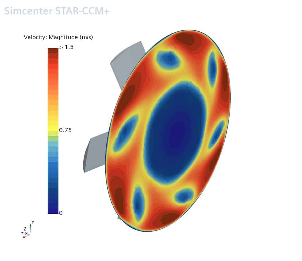
All this being said, we can compare the steady-state MRF flow field (right picture below) with an instantaneous snapshot of the RBM flow field (left picture below) where the fan positions are identical. In this particular case we can see that the MRF seems to predict the average flow field fairly well.

When to use what?

So which approach should you choose for your rotational flow problem? In short, the answer depends on the objective of the simulation, the timeframe of the project and the (computational) resources available. There are however some general recommendations when it comes to physics and type of application. For example, the MRF approach typically performs a lot better for axial impellers than radial impellers. For more information on this Siemens have actually provided a short summary on the topic here Should I use moving reference frames or rigid body motion for my simulation? (siemens.com).

We at Volupe hope this blog post was helpful to show how you can model rotational flows in Simcenter STAR-CCM+. If you have any questions or comments you are always welcome to send them in to support@volupe.com.