Sometimes you have simulation results that would be helpful to use as a starting point for another simulation. Perhaps you want to fine tune a boundary condition but save time by using a better starting guess, or maybe you want to run a single phase simulation and use the solution to initialize a multiphase case? In this week’s blog post we will go through how to achieve an initialization with an existing solution using tables in Simcenter STAR-CCM+.
Required input for initial conditions
Let’s start with looking at the required input for the initial conditions of a typical fluid flow simulation. For this example we’ll consider a three-dimensional single phase turbulent flow. In a case like this you’ll need to specify initial conditions for pressure, velocity vector components (i, j, k) and turbulence quantities.

This means that we need to extract these field values in each and every cell of our existing simulation – and to do so we will use a table.
Extracting field values using a table
To extract the field variables needed we create an internal table, most commonly an XYZ Internal Table’. Inside the ‘XYZ Internal Table’ context we select the field variables we want to extract from the simulation. X, Y and Z cell coordinates will follow by default.

Inside the table properties, click the ‘Scalars’ selection field to open the scalars selection dialog box.

The Scalars selection dialog box includes a search field (‘Filter Pattern’) to help filter out the variables you’re looking for. Note that the ‘Filter Pattern’ is case sensitive. In our example the ‘Scalars’ selection should look something like this (selected scalars in the rightmost column):

Now we extract the variables by right-clicking the table and select “Extract”. You will see that the ‘Extracted’-field becomes populated with the scalars you selected . These values are now ready to be used as initial conditions in the current simulation. If you wish, you may also export your table in .csv-format to be used as input in a different simulation.
Setting up the initial conditions with the tabulated values
Now, let’s set up the simulation using the exported field values as initial conditions. We move into the ‘Continua’ folder and navigate down into the ‘Initial Conditions’. Now we may choose ‘Table (x,y,z)’ as our input of choice for the different properties.

Once we make this selection, the field variable node turns into a folder where we can navigate down to the ‘Table (x,y,z)’ node. Inside this node we select the table we want to use for input (I.e. ‘XYZ Internal Table’) and the field variable associated to the initial condition (in this case ‘Pressure’). As mentioned above, the cell coordinates follow by default.

Now you may simply repeat this setting for all field variables. Note that the default input for turbulence quantities for a case like this using a two-equation turbulence model (e.g. k-epsilon) is ‘Turbulence Intensity’, ‘Turbulent Velocity Scale’ and ‘Turbulent Viscosity Ratio’. However, these quantities are not available for selection among the predefined field functions. Remember, we chose to extract the ‘Turbulent Kinetic Energy’ (k) and ‘Turbulent Dissipation Rate’ (ε). So how do we use these quantities instead? The solution lies within the ‘Turbulence Specification’ node. Here we can change the way we want to specify the initial conditions of the turbulence quantities. In this case we want to change to ‘K + Epsilon’.

Now we are ready to use our extracted field variables also for the turbulence quantities.

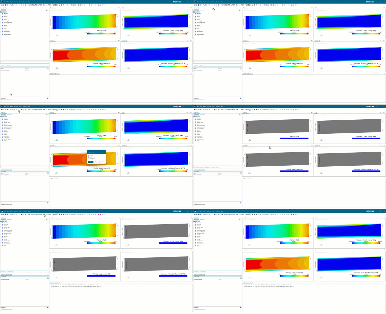
Once we have referenced all our initial conditions to the tabulated values, we can clear our solution and hit the ‘Initialize’ flag to see the tabulated solution popping up.
I hope this blog post was helpful to show how you can use an existing solution as input to a new simulation run in Simcenter STAR-CCM+. As always you are welcome to send any questions or comments to support@volupe.com.
Author

Johan Bernander, M.Sc.
support@volupe.com
+46 702 95 18 31


