Overset mesh in Simcenter STAR-CCM+

Download the simulation files which correspond to the two videos in this blog post:
[wpdm_package id=’5503′]

This week at the Volupe blog we will look into the exciting area of overset meshes. Overset mesh is a method using (at least) two different computational grids, and allowing the grids to overlap and transfer flow field information between the grids. Usually one mesh is describing the whole computational domain (background mesh), and the other mesh is describing the mesh for a smaller part of the domain which is moving with an moving object (overset mesh). The background mesh is usually quite coarse while the overset mesh is refined, since the moving object may need a customized refined mesh to predict the more complex flow field around it. One example where overset mesh comes in handy is when simulating a football moving through air, as in the picture below.

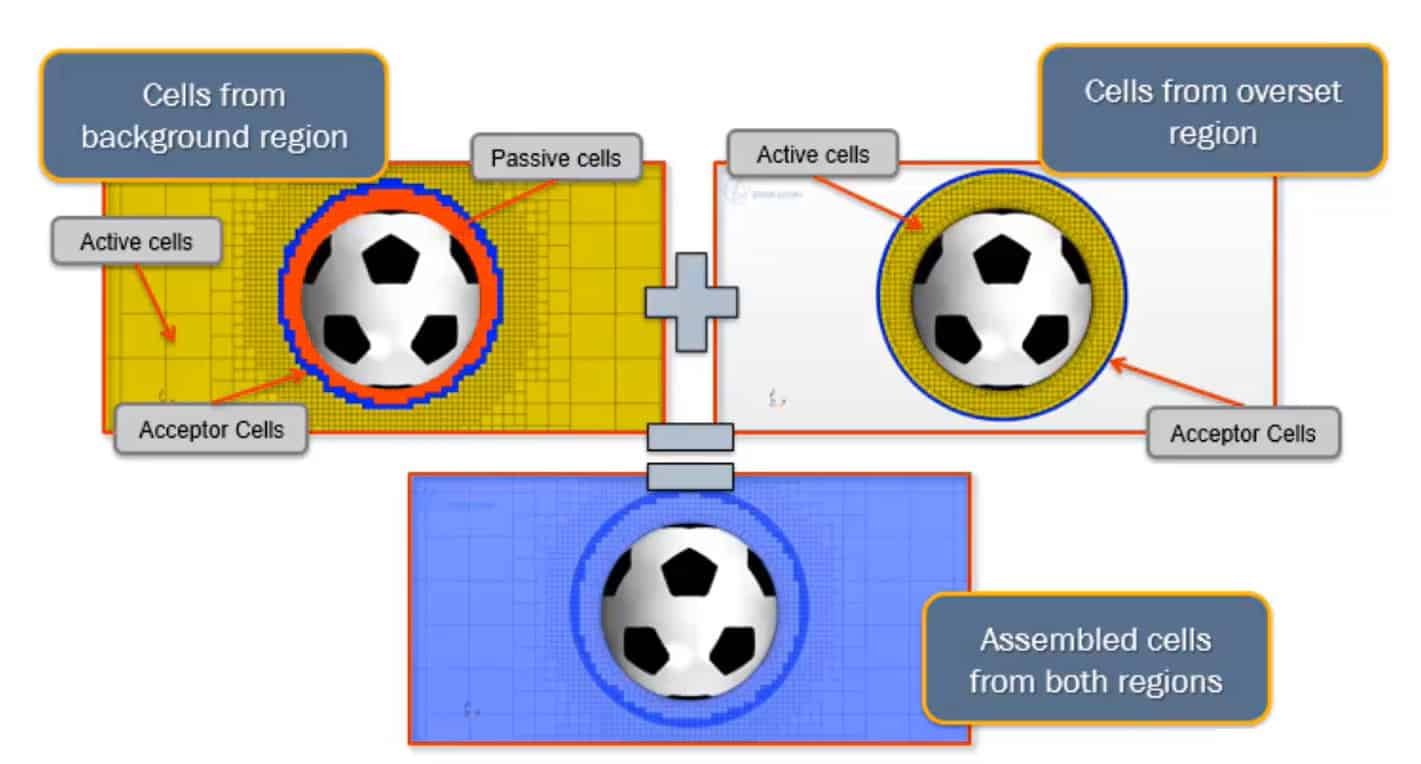
In the picutre above you can see the regions descretized by the background mesh, overset mesh and also the mesh which will be used by the simulation – the assembled mesh (displayed with light blue colour in the picture). There is a colour coding in the picture to describe which cells transferring flow field information:

Yellow – active cells. It is in these cells which the flow equations are solved. Active cells are present in both the background and overset mesh.
Blue – acceptor cells. These cells are transferring data between the background and overset mesh. Acceptor cells are present in both meshes. When a cell is receiving data it is named “acceptor” and when it is providing data it is called “donor”.
Red – passive cells. Cells where the flow equations are not solved are called “passive”. One example of where passive cells can occur is in the background mesh where the overset mesh cells are used in the assembled mesh.

How to create an overset mesh region

In Simcenter STAR-CCM+ overset mesh is a type of boundary condition for your region. A region is a discretized domain in your simulation. If you have the example of the football, the background region will be using the background mesh, and the region enclosing the football and the air around it will be in the overset region using the background mesh. In the picture below you can see how it looks when the outer boundary of your overset mesh is using the boundary condition “overset mesh”.

After setting the correct boundary condition, you can create the coupling to the background mesh. Select both regions, then right-click and choose “create interface”. Here you select the wanted type of overset mesh – “overset mesh” or “overset mesh zero gap”, as visualized in the picture below. Overset mesh with the zero gap feature can create temporary walls between regions in order to close small gaps, which is useful when surfaces will come into contact.

Dynamic overset behaviour

When using overset mesh, the object is supposed to move within the boundaries of the background mesh. The overset boundary can however be partly outside the background mesh. If so, the cells that are outside the background mesh will be inactivated.

There is a possibility to allow the computational region to be extended if the overset region moves outside the background mesh though. This works for overset meshes that are sliding on the background regional outer boundaries as well. An example of this can be if you have a train which is moving, and you want to have a mesh resolution which is customized for the ground and air below the train.

To activate this feature you set up your simulation with the overset mesh interface as described in the previous section. The boundaries with overset mesh boundary condition (boundaries related to the overset mesh interface) should be set as wall. For both the boundaries related to the overset mesh interface and the outer boundaries of the background mesh that will come in contact with the overset mesh region, the “dynamic overset behaviour” should be set to “Active, Acceptor”, as seen in the picture below.

These settings will generate a simulation as described in the video below.

If the region is not supposed to be extended, but the object is supposed to be moving outside of the domain, overset mesh with zero gap can be used. See video below for how the generated simulation will look like with these settings. In this simulation the overset mesh region uses overset mesh boundary condition at the interface, and dynamic overset behaviour is kept as default “Active, inactive”.

Golden rules for overset mesh by Siemens

There are a lot of settings, and therefore possibilities for overset meshes. Siemens has provided a comprehensive “Siemens TV broadcast” on overset mesh, linked here, to explain how to use overset meshes. This TV broadcast has been used as a source of inspiration to this blog article. In the TV broadcast the so called “golden rules for overset mesh” are explained. Below we summarized the golden rules and the tips provided by Siemens:

In locations where you have acceptor cells the background and overset mesh should have as equal cell size as possible. It is therefore recommended to have the same cell size in the outer part of the overset mesh as you have in the background mesh. This can be obtained by including all parts included in both regions into the same mesh operation and use “per-part meshing”. Specific surface and volumetric controls can then be added to customize the mesh for the overset mesh. If you encounter problems using per-part meshing it can be better to copy the mesh operation and have two different operations for the two meshes. By copying one mesh operation when creating the second the settings will be identical in the two operations.
It is recommended to have at least 5 cells over the location where the meshes are overlapping. If you don’t have enough cells here, a refinement of the mesh might help.
The overset mesh feature “close proximity” can make the interpolation work with 2 cells instead of 5 in the overlap. Close proximity is a feature activated at the interface. Cells in the overset mesh that are outside of the background mesh will be deactivated (passive cells).
The overset mesh feature “alternative hole cutting” can control which cells that are active and inactive, which might help in the simulation. Alternative hole cutting is activated at the interface.
In time dependent simulations (which are standard when running overset mesh simulations) the Euler scheme order for the solver will set limitations on how the overset mesh can travel. 1st Euler scheme order allow cells to travel as far as the smallest cell in the region. If using 2nd order Euler scheme will allow cells to travel half the distance of the smallest cell in the region. If the time step is too large the cell will travel too far, resulting in holes in the mesh. This can be solved by either decreasing the time step or coarsening the mesh.
If further debugging is needed, please take a look at this video article, linked here or by reading in the documentation at Simcenter STAR-CCM+ > Simulating Physics > Mesh Motion and Adaption > Overset Meshes > Overset Mesh Reference > Overset Mesh Field Function Reference.
When running overset mesh simulations the partitioning is recommended to be set to “per-region” for the solvers. This might both make the simulation more stable and speed up the iterations.
Also keep in mind that mesh-morphing together with remeshing can be a good alternative to the overset mesh strategy.

We at Volupe hope that this blog post about overset meshes has been interesting and that it will help you in your work as an engineer. And don’t forget that you are always welcome to reach out to us at support@volupe.com.