As a Simulation engineer you always compromise between computational power, mesh size and accuracy. Thankfully we have the Adaptive mesh refinement (AMR) as a dynamic method to refines or coarsens cells based on adaptive mesh criteria as they query the flow solution. Such that we can have a fine mesh only where we need it, at the point in time we need it. This feature was introduced to Simcenter STAR-CCM+ already 2020. But still there are some deployments of AMR to discover. Let’s find out how you can spatially restrict the VOF model driven AMR to resolve only specific flow feature in this week’s blog post.
Adaptive Mesh Refinement
AMR refines the computational mesh dynamically only in areas where needed i.e., to capture the relevant flow features while recovering coarser cells elsewhere. The model-driven AMR refines the mesh automatically with minimal user intervention until the final accuracy levels are met. Two general types of adaptive mesh criteria are available:
- Model-Driven Mesh Adaptions, where the adaption criteria are provided automatically from the Simcenter STAR-CCM+ models. Currently the following options are available:
- VOF
- LSI
- Overset Mesh
- Reacting Flows
- User-Defined Mesh Adaption, where you provide a field function or a table that prescribe how the AMR solver is to drive mesh adaption.
AMR driven by the multiphase Volume of Fluid (VOF) model allows to refine coarse cells ahead of the free-surface. It is actually superior to traditional field functions based refinements in capturing the air/fluid interface. Because the model-based free-surface AMR anticipates even the movement of the free surface.
However, sometimes you are not in the need to apply AMR in the entire domain. Because static mesh refinements based surface and volumetric controls are sufficient to capture the flow. One such case would be calm water resistance calculation of ships. The VOF interface in such simulations is to a large extend flat and the zone where waves are expected to build up are rather small predictable.

But what if, there is a specific behaviour at the VOF interface that you want to resolve more detailed? This could be a vortex, ventilation, or breaking waves. You can of course define a volumetric refinement in; in case you know where the entity develops and where it evolves. In most of the cases your refinement zone will, however, end up to be too large or overly complicated.
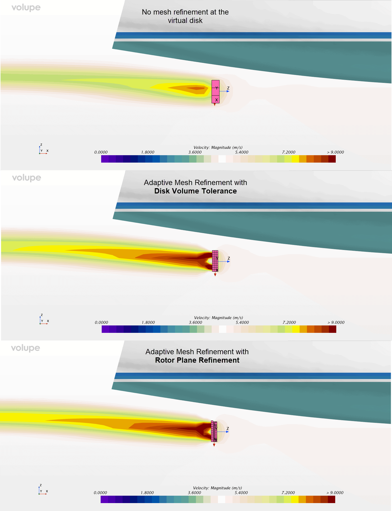
This is the core application area for ARM. If you still want to restrict the propagation of refinements in your domain, you can restrict AMR on a single region (if you have several). An example is the “Example of yacht manoeuvring in waves with tight-overset approach and AMR”. Here we use a sufficiently fine grid in the overset region (yacht) and refine the background regions with both VOF model and Overset Model driven AMR. In the overset region, the mesh adaption is disabled (Overset Domain > Physics Condition > Adaption Option).

Local AMR restriction
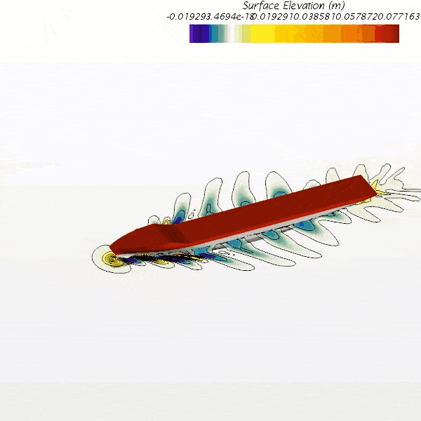
Let´s take the example of yacht that develops a significant bow wave. The setup is taken from the Marine Self-propulsion tutorial and is essentially indicating a typical calm water resistance simulation with refinements for the waves (see image further above), yet no mesh adaption.
We will now try to resolve the bow wave with AMR in a region around the bow (see below). The VOF Model-Driven Adaption would refine the interface in the whole domain. Therefore we use User-Defined Mesh Adaption and define a Field Function that is only returning a value inside the desired area (see below).

The restrictions in three-dimensions can be defined in Field Functions with the help of $${Position} vector and a condition. Please refer to https://volupe.se/star-ccm-field-function-syntax-part-1/ for detailed description on Field Function syntax.

For a two-dimensional case we can easily restrict the refinement between -50 and 50 m in x-direction with the help of the syntax above.

The volume fraction suggests itself to be a valid field to trigger mesh adaption. However, in most cases the volume fraction is too sharp to trigger the mesh adaption. Better distribution can be obtained for the adaptive refinement based on second gradient of volume fraction.

The final Field Function to define the region around the backboard side of the yachts bow reckons as:
($${Position}[0]>10 && $${Position}[0] < 14 &&
 $${Position}[1]>0  && $${Position}[1] < 3  &&
 $${Position}[2]>-0.5 &&  $${Position}[2] < 0.5) ? div(grad(${VolumeFractionwater}))*${AdaptionCellSize}:0

Together with the adaption properties as follows. The Range [-1.0, 1.0] where to keep the original mesh may vary depending on the ${AdaptionCellSize}.
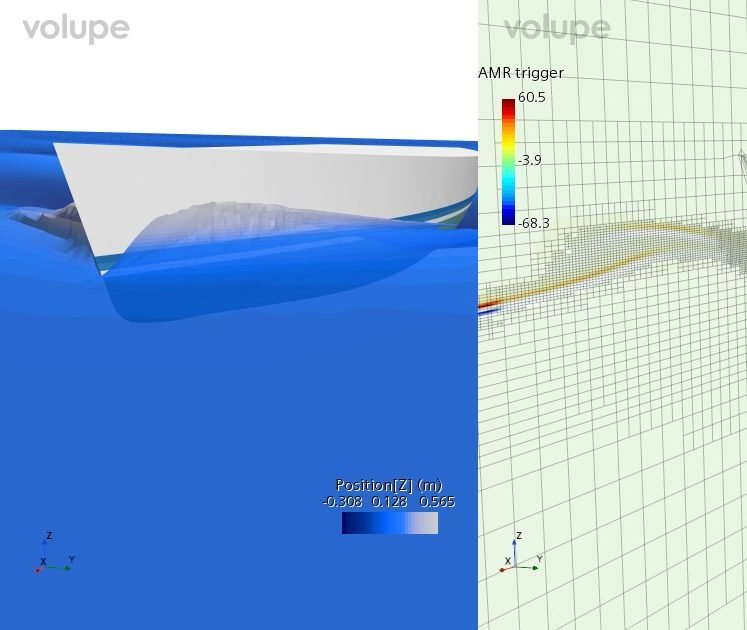
With those settings we finally get the simulation which only refines waves only at the backboard side of the yacht. Yet, only in vicinity of the VOF interface. The plot of the wave-cut on backboard and starboard clarifies the effect of the local wave refinement.

We hope the topic of this article is interesting and may help you reach your goals with Simcenter STAR-CCM+ faster. Please find attached an example implementation of a User-Defined Mesh Adaption for VOF interfaces. If you have any questions or comments, please feel free to reach out to us on support@volupe.com
[wpdm_package id=’6774′]
The Author
Florian Vesting, PhD
Contact: support@volupe.com
+46 768 51 23 46