Last week we investigated at the basic field function syntax in Simcenter STAR-CCM+. This week we will keep looking at the possibilities of the field function syntax and see what else can be done. Last time we focused on spatial limiting for initial conditions in terms of temperature. The scalar is arbitrary, so we will look beyond the spatial discretization here and look at writing field functions depending on other physical quantities than space. Meaning that we will not limit ourselves to position. We will also investigate at how to interpolate data from a table.

Ramping time step

In the beginning of a transient simulation, it is often a good idea to advance slowly in time using short timesteps and increase the timestep size gradually. A simple linear ramp of the timestep can be written as shown in the picture below. Here, the time step is linearly ramped up to 0.1 s from simulation time 0 to 1 s.

Again, we assign a value based on an if-statement. We say that if time is smaller or equal to 1 second our timestep is 0.1 times our actual time plus an additional 1e-4 s. And while the time is larger than 1 s, our timestep is instead 0.1 s. The additional 1e-4 s is added to have a valid timestep when the simulation starts. Otherwise the first timestep would be zero and the simulation would not start stepping forward in time. If this is the case, you will get an output warning saying that the timestep must differ from zero.

This simple expression has now allowed us to ramp the timestep and that will hopefully either stabilise our solution or can be used to resolve an actual small time-scale event. (${Time} <= 1 ? 0.1*${Time}+1e-4 : 0.1)

Interpolating table values

Instead of creating our own expression, we can also use table values. Assume we have a table with values, and we want to use that information as inlet temperature at a boundary in our simulation. The simple example table used here is shown below, a quadratic relationship between input (time) and output (Temperature).

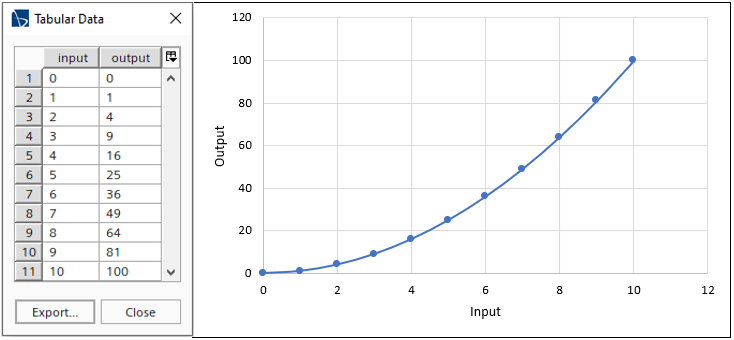
We then write another field function referencing the table we have created, here named my_table. In our previous example we ramped our timestep with a linear relation using only field function syntax. It this example we interpolate the temperature inlet value using table values instead and now use a quadratic relation for our output (the temperature).

Note also that a table interpolation exceeding the input value of our table (max 10) will still give the highest value from the table, since in this example the expression still employs interpolation from the table. Meaning that if you run up to the value of 100 (for more than 10 seconds), there is no explicit need to express what happens once time exceeds 10 s. (interpolateTable(@Table(“my_table”), “input”, LINEAR, “output”, ${Time}))

Combining interpolation and statement

Assume instead that we have a step function like input data in our simulation according to the figure below. In this graph there is a large change in data input at around every 30 seconds. We wish to run our simulation with a timestep of 1 second, but at around the abrupt input changes we would like to set the timestep to 0.1 s. This to deal with whatever impact the change has to our simulation. Assume also that we would like a rather general expression for this. This will require our expression to look forward in the input data and see whether to reduce our timestep size or not, because we want our timestep to be reduced before and not after the abrupt changes take place. So, how can this be done? Since we can look forward in the input data table, we can base our timestep size on the future input data value of our simulation. We can see from the graph below that when large changes in output happens the absolute change exceeds at least 1. At the high and low locations in our graph, there are still changes in output, but it rarely exceeds 0.1, hence the absolute value on the change of 1 is a safe value.

So, what we do is compare the current timestep we are at, the interpolated table value at Time=t with the interpolated table value of Time=t+1. If the change is larger than 1, we reduce the timestep size to 0.1 s. The full expression and the preview can be seen in the figure below. (${Time} == 0 ? 0.1 : abs((interpolateTable(@Table(“data_table”), “time”, LINEAR, “Value”, ${Time}) – interpolateTable(@Table(“data_table”), “time”, LINEAR, “Value”, ${Time}+1))) > 1 ? 0.1 : 1)

So, what is done is a comparison of the absolute output value of the current timestep compared to the output value in 1 second. And if the difference exceeds 1 the timestep size is reduced to 0.1 s.

There are two if-statements, where the second one is called upon if the first one’s specific request for time == 0 is not fulfilled. Then the second one compares the difference in output for current time and output one second later. And if the absolute value is larger than one, the timestep is set to 0.1 otherwise it keeps the value of 1. The time step size is also lowered slightly before the change in output happens. The amount of time the timestep is lowered can be reduced by reducing the time ahead you are looking at the output value.

I hope this has been useful. As usual do not hesitate to reach out to support@volupe.com if you have any questions.