The applications for creating mathematical models to approximate behavior in data from simulation or field-testing measurements are numerous. Not only can these models be used to conveniently query information about the state of a particular sensor in a large set of transient sensor data, but also provide a means for assessing where a simulation model is prone to error. By incorporating a mathematical representation of a test-object directly inside Simcenter Amesim comparisons can be made instantaneously. The modeling possibilities are not limited there however. Arguably the greatest potential is seen in the way this approach can be combined with the use of physics-based modeling to allow for evaluation of control strategies and software features at very early design stages, in real time.
In this blog article we exemplify the process of Reduced Order Modeling (ROM). A dynamic time dependent neural network was constructed using Simcenter Amesim’s ROM Builder and based on dynamic simulation data provided by Simcenter Amesim. Although we limit ourselves to system simulation in this post, data generated from other sources such as CFD, FEA, and testing can also be managed by the tool. For a general overview of the ROM Builder please refer to this earlier blog post here.
Reduced Order Models are often seen as computationally inexpensive mathematical representations that provide the potential for near or real time operation. Though most of these models perform in real time, creating them can however become computationally demanding as they require sufficient input data characterizing the underlying behavior of a simulation or measurement. Moreover, due to the mathematical model’s inability to account for changes made to test objects or simulation models, ROMs usually have to be reconstructed for each significant variation.
These two issues emphasize the need for a simple and versatile framework to quickly develop and deploy ROMs. Although many approaches for creating mathematical models from data exist, e.g. Python used together with TensorFlow. Not all of these are easily managed and may require extensive know-how to properly set up. By working through Simcenter Amesim, and its integrated ROM Builder, models can be created from simulation results, evaluated, and then exported to other tools by a step-by-step process. If changes are done to the underlying system, previous simulation settings and case definitions may be reused to produce a new set of results later imported into ROM Builder.
The process, step-by-step
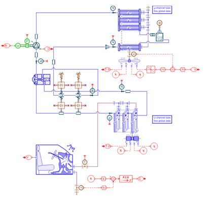
To illustrate the dynamic modelling features in Simcenter ROM Builder, the demo-model titled “Reduction of an air conditioning system” was used to conduct several transient simulations. The following example, and all accompanying files, can be found within the documentation of the tool.
The dynamics of the AC system model were investigated by simulating vehicle speed as an input to influence air velocity across the system’s condenser. Vehicle speed was varied using a few predefined driving cycles commonly found in the automotive industry. Alongside vehicle speed, the following three parameters were also used: Ambient temperature, Compressor speed (given by gear profiles matching the driving cycles), and Compressor command.
Although three outputs/system-responses are defined in the example we proceed by only focusing on the outlet temperature of the evaporator.
Simcenter ROM Builder is found and started from the App space menu, and for this exercise a time-series based project was selected. By doing so Simcenter ROM Builder is configured to conserve the time-dependent relationship between inputs and outputs. We proceed by doing some bookkeeping and update the Alias list with the names of the driving cycles for future reference before we import.
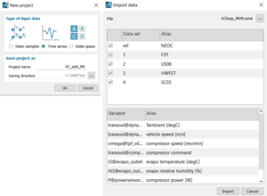
Next, a selection is required regarding which dataset/datasets to use for training, validation, or left unused. As the generalization and resulting accuracy of a neural network is usually improved by allowing the training process to work with a wider ranging and more varied dataset, it is advisable to invest time and thought into setting up the underlying experiments/simulations. Additionally, it is important to establish how the ROM is intended to be later used. As with most modeling, the statement; ”garbage in, garbage out”, or bad inputs produce bad outputs, is also applicable to neural networks.
Regarding model inputs and outputs, it is again recommended to consider future use. Since the simulation results were created using all four inputs it is likely, but not certain, that all four are required to explain the behavior of the outputs. Simplification, and potentially reduction of disturbances in the final model, could be achieved if some of the inputs are found to have a week link to the output. Furthermore, it could be worth considering if a single model should predict the behavior of all outputs, or if instead several models could be created containing only a single output each. The later would possibly simplify the network configuration and offer more precise predictions., but at the price of managing several neural networks.
Proceeding with model creation, the built-in wizard was used to recommend a neural network architecture. The tool automatically configures the input and output layers corresponding to number of specified inputs and outputs, and a recommendation is given for number of hidden units between these layers. Additionally, settings for model hyperparameters are also proposed which involve the type of neural network to be used in each layer, neuron activation functions, and number of neurons in each layer.
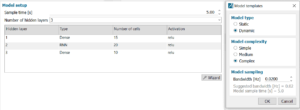
In our case a depth of three hidden layers is proposed, containing two dense layers with an intermediate recurrent neural network (RNN). Each layer contains between 10 – 20 neurons. Using only fully connected layers (dense) would result in a very versatile network, well suited for approximating and mapping almost any static relationship between inputs and outputs. Applying a recurrent neural network to these layers allows the network to approximate time dependent relationships. This is done by using sequential information from earlier inputs in a timeseries to affect the current input and output. An illustration of an RNN is provided below.

Apart from RNNs, other network types are given as options. Gated Recurrent Unit (GRU) and Long-Short Term Memory (LSTM) may improve a neural networks ability to predict slow dynamics if this behavior is present in a dataset. These can either be combined with or used to replace an RNN.
An additional aspect when creating dynamic neural networks with Simcenter ROM Builder is related to sample time, i.e. time step or output frequency of the resulting dynamic network. For static networks the choice of sample time influences the amount of training data made available for training. Using a sample time corresponding to the imported data set, in our case 0.25 [s], would result in training with all available data in that set. This may not always be necessary and therefore downsampling can be achieved by selecting a larger sample time.
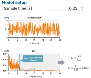
For dynamic networks, time sampling not only influences the amount of data used to properly identify and capture dynamic performance, but also affects the feedback loop of the RNN. Decreasing the training sample time would allow the network to consider more information but may result in an overly complicated network which may still be unable of predicting the overall dynamics in the data. It is worth considering if any underlying noise, or high frequency dynamics not deemed necessary, can be reduced in order to simplify the training process. A starting point for sample time is automatically suggested by the wizard using a process involving Fast Fourier Transformation (FFT) to determine a suitable maximum frequency. The process is outlined in the figure below.
To demonstrate the outcome of working with insufficient training data. The dataset titled WHFET (EPA Highway Fuel Economy Test Cycle) was selected for training while the other datasets were left unselected. The New European Driving Cycle (NEDC) was selected as the validation set and used for later comparison. The limitations of using WHFET to approximate behavior in NEDC is illustrated in the following figure, where the input variable Vehicle Speed of both sets are given.
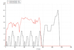
As seen, the vehicle speed of HWFET (in red) is predominantly high throughout the entire cycle. As opposed to the validation set NEDC (in black), where a more limited high-speed portion is located towards the end of its cycle. This has the implication that a model trained with this set will perform poorly if used for studies in the NEDC speed range.
The result from a network containing only the Evaporator outlet temperature as output is given below. The model was trained for 500 epochs, i.e. iterations containing the entire dataset in each step, and used default training settings.
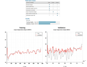
The leftmost graph above displays training results by comparing model predictions (red) with the true values in HWFET. The training data’s behavior was to some extent replicated by the network. The same can however not be said for the validation in the rightmost figure. Evident by the trained networks inability to predict the lower temperatures found in NEDC, and by struggling with the overall dynamics of the response. Only the high-speed portion at the end of the cycle is to some degree within range.
The HWFET – NEDC comparison is a very simple example of using inadequate information for constructing a ROM, and typically more considerations have to be taken into account when determining input data. Apart from a varied range, limiting repetition is also important as the resulting network will become more heavily weighted towards repeating data points. This is usually undesirable in a neural network as the generalization, and thereby its general applicability, decreases. Introducing time dependent behavior to a neural network also involves investigating the dynamic properties of a data set. As an example, consider the rate of change for Vehicle Speed above. Here it is prudent to ensure that the expected range for both acceleration and deceleration is well represented within the training data.
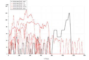
Continuing onwards. The neural network was retrained using all remaining training sets, and as will be seen, the resulting predictions drastically improve by doing so. Below, vehicle speeds of all datasets are given to visualize the increase in variation experienced throughout training.
In the subsequent three graphs, a comparison between model prediction and the true output values of NEDC are provided. The leftmost graph contains results from the model trained only using the HWFET set, and is the same plot as shown before. The middle figure is the outcome of training with all available training sets, and the last figure contains predictions made by a network trained with all data as well as modified hyperparameters.
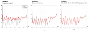
Once more datasets were added to the training, the network’s ability to capture the dynamics was greatly improved. This is clearly seen by comparing the prediction made in the leftmost figure with the prediction of the middle figure.
To further improve upon the model, a brief investigation into model hyperparameters was carried out. The sampling rate was decreased, an additional fully connected layer was added in front of the RNN, and the number of neurons in each layer was doubled. Comparing between the middle figure and rightmost figure, some improvement can be seen in the low temperature range. It is however reasonable to suspect that the underlying data does not contain sufficient low temperature data to fully describe this behavior, and arguably that any further hyperparameter tuning will only result in marginal gains.
Closing remarks
Creating dynamic neural networks using an easily manageable interface such as Simcenter ROM Builder offers several benefits. Reasonable results can be achieved without requiring considerable effort, and the connection to Simcenter Amesim provides the possibility for quickly retraining networks once new data becomes available. Additionally, and although not discussed in this post, exporting models to other tools can also be done through the use of the FMI and ONNX frameworks.
As more and more control software and product features find its way into our products, early software testing during product development becomes increasingly important. A realistic way of achieving this involves levering the real time capabilities of dynamic neural networks with the underlying flexibility and accuracy of physics-based models.
Hopefully you found this post interesting. If you have any questions or comments related to the topic, or regarding simulation in general, please feel free to reach out.
Author
Fabian Hasselby, M.sc.
+46733661021
fabian.hasselby@volupe.com


