Turbulence for multiphase simulations in Simcenter STAR-CCM+

Last week’s blog post was about transition modelling in Simcenter STAR-CCM+. I was thinking that this week we keep working with turbulence in Simcenter STAR-CCM+. Specifically, I will discuss multiphase turbulence and how that is treated, and even more specifically, how to simulate turbulence in your Eulerian multiphase simulation (EMP). Back in version 2021.1, mixture turbulence was introduced as an optional appoach instead of doing EMP simulations. We will look at what that means, in terms of the details for the transport equations of turbulent quantities. I will go over the options for dispersed phase turbulence, response models and turbulence interaction. This can actually be a bit confusing, so I hope that this blog post can help sorting out some of the difficult areas. Examples of the different methods will be presented using the k-epsilon turbulence model or a generic turbulent quantity. Details for other turbulence models can be found in the Simcenter STAR-CCM+ documentation.

Mixture turbulence

For mixture turbulence, a single turbulence model is used to calculate the turbulence of all phases by solving the turbulence quantity transport equations using mixture properties and mixture velocities. Doing this in your EMP-simulating you are nearing the approach of using the MMP model, especially in terms of turbulence modelling. Other properties used in fundamental equations (mass, momentum, and continuity) are still summed up over the separate phases rather than being treated as mixture properties. The turbulence models that currently (in version 2022.1) support mixture turbulence are the k-epsilon, k-omega and Reynolds stress models. Both mixture density and mixture dynamic viscosity is calculated using linear interpolation of the quantities of all other phases weighted by the volume fraction. Turbulent kinetic energy is the energy per mass of the velocity fluctuations, so it is assumed that the mixture k and phase k are equal. Also, the dissipation rate density is assumed to be equal for the mixture and the phase. The calculation of the mixture turbulent eddy viscosity assumes that kinematic viscosity of the phases is equal.

The option of using mixture turbulence improves stability to the simulation by reducing the degrees of freedom of the system being solved while also reducing the number of transport equations that require solving (in two-equation turbulence models the reduction will be two equations per phase). The mixture turbulence is especially beneficial for applications involving bubbly flow where turbulence is mainly a function of the heavy phase. For such a case, it presents unnecessary overhead to calculate the gas phase (bubbles) turbulence separate. The bubbles will be carried with the liquid and respond to the heavy phase turbulence. The phasic turbulence is more accurate when the dispersed phase describes the heavy phase, but more on phasic turbulence below. The conclusion is that applying mixture turbulence in your EMP simulation, applies turbulence in a similar fashion to Mixture multiphase (MMP).

Phasic turbulence – continuous phase

When discussing phasic turbulence, it is relevant to mention the continuous phase turbulence, regardless of if we have an actual dispersed phase/continuous phase or multiple flow regimes. For the continuous phase, Simcenter STAR-CCM+ solves two modified transport equations for turbulence quantities. Those modifications include the volume fraction of each phase and additional source terms that account for the effect of the dispersed phase on the continuous phase turbulence field.

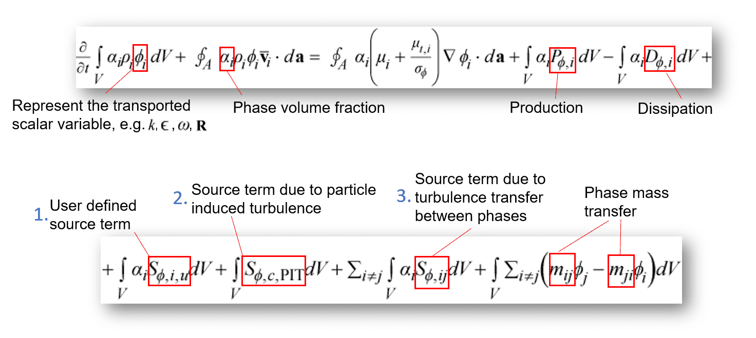
The production and dissipation terms vary based on the selected turbulence model. It is the source terms (1-3) here that are of special interest. Their existence of the source terms in the turbulence equations is based on some different selections, the separate terms are described below:

This is a user defined source term.
The source term due to particle induced turbulence is representing turbulence implemented from dispersed particles. It only enters the continuous phase transport equation.
A source term due to turbulence transfer between phases, the effect on turbulence from drag. (More on this under the section of interphase turbulence transfer).

Note that these transport equations are always solved for the continuous phase. They can also be solved for the dispersed phase, if you do not use a turbulent response model.

Phasic turbulence – dispersed phase

As was just mentioned, the dispersed phase turbulence can be calculated using the same equation as for continuous phase turbulence, except for the source term relating to particle induced turbulence (number 2 in the picture above in the previous section). The other option is to use a semi-empirical model to correlate the turbulence from the dispersed phase on to the continuous phase (response models). The full turbulence model for the dispersed phase is recommended to use when you have mixed regimes (when the primary and secondary phase are both the dispersed phase at different spatial locations, e.g., droplets in air at some locations and bubbles in water at other), or when you have heavy particles where a large portion of the kinetic energy is held by the dispersed phase.

We can use a response model when we have a clearly defined dispersed phase, and the response model will then provide the effect the dispersed phase effective turbulent diffusivity and standard wall-functions.

Response models

The turbulence response models predict velocity fluctuations in the dispersed phase using algebraic correlations to the velocity fluctuations in the continuous phase. The turbulent stress is modelled using the eddy-viscosity concept. The below picture explains, again in terms of the k-epsilon turbulence model, how the response function is used to calculate the turbulent kinetic energy and the dispersed phase turbulent eddy viscosity. It is the term response function (C_t) that requires a closure model.

Simcenter STAR-CCM+ hold two such response model that are needed here. I will not go over them in detail (the equations) for brevity, details can be found in the documentation:

The Issa response model defines the response coefficient (C_t) with a volume fraction correction. It provides the response coefficient for bubbly flow.
The Tchen response-model provides the dispersed phase turbulent diffusivity for gas flow laden with heavy particles.

Particle induced turbulence

The particle induced turbulence models add more source terms to the continuous phase turbulence kinetic energy and dissipation equations. The models represent modification of turbulence due to the presence of a dispersed phase. The different model here works a bit differently, again, for brevity we will go into the details. The models generally enter the modified turbulence transport equation in the source term relating to particle induced turbulence (The source term 2 from one of the pictures above).

The Troshko Hassan model describes bubble induced turbulence effects.
The Gosman model uses Reynolds averaging of the continuous phase velocity fluctuations times the drag source term from the fluctuating part of the continuous-phase momentum equation to provide a source to turbulent kinetic energy.
The Tchen model work like the Gosman model but introduces additional terms to account for more regimes.
The Sato model does not provide Source terms, but instead considers the turbulence effects of the dispersed phase on the continuous phase in the form of an enhanced effective viscosity. It is the earliest and simplest model for particle induced mixing and provides a robust alternative to the later source-based methods. It is applicable for dilute bubbly flows.

Interphase turbulence transfer

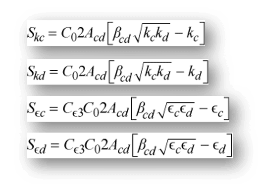
As if it was not enough with response models and particle induced turbulence additions to the turbulent quantity transport equation, you can also include interphase turbulence transfer. This is a property selected in the multiphase interaction model in Simcenter STAR-CCM+. What it does is to account for the contributions to the fluid and particle turbulent kinetic energies due to drag. It is only available when the continuous phase is a gas and the dispersed phase is made up of solid particles. Moreover, the model is best applicable when the particle size is between 20 and 100 microns and have a density lower than 1.4 g/cm2 (a typical application is Fluid Catalytic Cracking, FCC). It is also only available when both phases use the k-epsilon model. The term that is modelled and require closure is the cross-correlation between fluid and particle fluctuating velocities evaluated along the particle trajectory. For k-epsilon the expressions looking like the below picture shows for the source terms of both turbulent kinetic energy and dissipation, for both the continuous and dispersed phases respectively.

The beta_cd-term is the velocity cross-correlation, which is set default as 0.7, but can be specified with any constant value, a field function, or with Zaichik Method (see documentation for details).

Turbulent dispersion

A particle in turbulent flow experiences a greater level of dispersion than in laminar flow. The turbulent dispersion force model then considers the effect on a dispersed phase particle from surrounding turbulent eddies. Such extra force, provide additions to both drag and virtual mass force.

Summary

Response models calculates velocity fluctuations in the dispersed phase based on continuous phase velocity fluctuations.

Particle induced turbulence represent modification of turbulence due to the presence of a dispersed phase.

Interphase turbulence transfer account for the contributions to the fluid and particle turbulent kinetic energies due to drag. Limited applicability!

Turbulent dispersion force account for the interaction between the dispersed phase and the surrounding turbulent eddies.

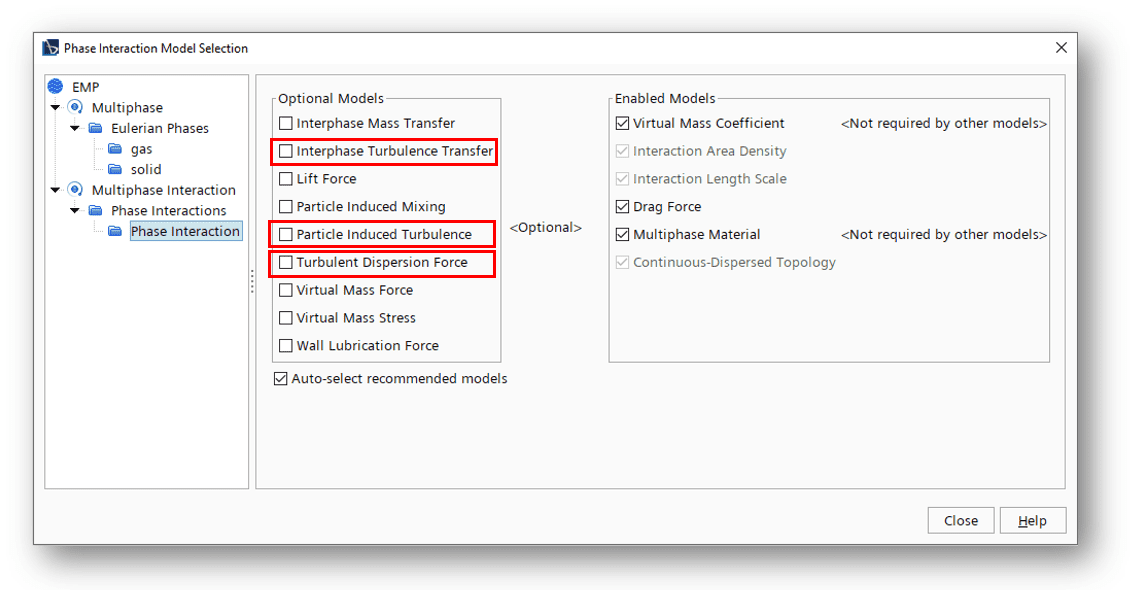
While the response models are selected instead of another turbulence model for a dispersed phase, under phase models, the Particle induced turbulence, the interphase turbulence transfer and the turbulent dispersion force are all selected under the phase interaction node in Simcenter STAR-CCM+. And for obvious reasons, of the methods mentioned above, only the turbulent dispersion force is available if you run the mixture turbulence.

I hope this has been useful when pondering how turbulence work when you are running a Eulerian multiphase model. As usual, reach out to support@volupe.com if you have any questions.